
| News | |
| QuikScat | |
| NSCAT | |
| YSCAT | |
| SAR Research | |
| SCP | |
| CERS | |
| Jason-1 | |
| Publications | |
| Software | |
| Studies | |
| Lab Resources | |
| Group Members | |
| Related Links | |
| Contact Us | |
| Getting to BYU | |
Point-wise Wind Retrieval
The most common method for scatterometric wind estimation is known as point-wise wind retrieval. In this method, the measured swath is divided into resolution elements known as wind vector cells (wvc's) and the wind is estimated independently at each wvc. The independent estimates are then processed to remove ambiguous solutions. The Geophysical Model Function To estimate the wind from scatterometer measurements, we must establish the relationships between the normalized backscatter and the wind speed and direction. This relationship is described mathematically by the Geophysical Model Function (GMF). Much research has been and continues to be done to accurately characterize the GMF. (See YSCAT and JPL). The GMF can be generically represented by the following equation:
The forward model function accepts as inputs: wind speed, relative azimuth angle (or the angle between the instrument azimuth and the wind direction), incidence angle, instrument frequency, and instrument polarization. The output is the normalized backscatter, sigma-0, or the measurement the instrument would return under such conditions. In general, the wind speed and the relative azimuth (which will be referred to hereafter simply as the wind direction) are unknowns, while the incidence, frequency and polarization are known for each measurement. It is important to recognize that the GMF accepts two wind inputs (wind speed and direction) to generate sigma-0. Unfortunately, the inverse model function is not unique. This implies that the inverse problem (i.e. deriving the wind vector from the measurements) is not trivial. Indeed, in the absence of other information, a single measurement generates a continuum of potential wind vectors, all of which would have given rise to the observed backscatter.

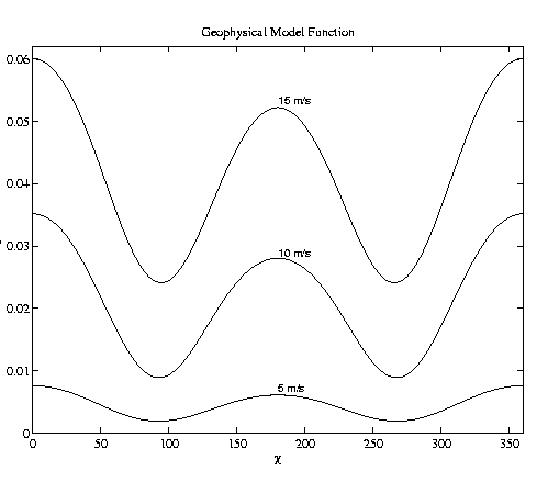
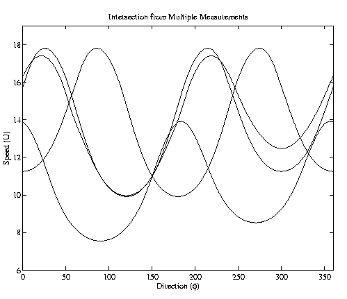
This figure demonstrates some of the characteristics of the GMF. For a fixed incidence, frequency, and polarization, sigma-0 is shown as a function of wind direction (x axis) and wind speed (labeled on each curve.) Note that in general, higher wind speeds generate more surface roughness and therefore higher sigma-0 values. We note that the model function has a cos(2X) symmetry. Although the problem has been studied for years, an accurate analytic derivation of the GMF remains beyond the current state of the art. Thus the GMF is typically empirically derived. The Point-wise Objective Function In order to resolve the inverse problem and solve for both wind speed and direction, multiple backscatter measurements are taken at each wvc. The following figure illustrates four different measurements (with different azimuth and incidence angles) taken with the same wind speed and direction. For each measurement, the figure shows a curve of the wind speeds and directions that could have given rise to the observed backscatter. Where the curves intersect is the wind vector consistent with the measurements.

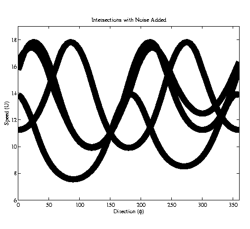
In the absence of noise, the different measurements allow the wind speed and direction to be resolved as 11 m/s and 150 degrees. Note however that there are near intersections at approximately 330 degrees, 40 degrees, and 235 degrees. The intersection shown is the idealized case where there is no noise in the measurements or the GMF. Unfortunately, the measurements are not noise free, so the problem becomes more complicated. In the presence of noise, the alternate intersections might appear to be more acceptable options.

Noise in the backscatter measurements is due to radiometric and thermal noise in the radar receiver and has an approximately Gaussian distribution. To generate a statistical model for use in estimation, each measurement is assumed to be a realization of a Gaussian random variable dependent on the wind speed and wind direction. Each measurement is assumed to be independent, thus the joint density function of the measurements given the wind vector is given by:

A maximum likelihood estimator for the wind vector can be formulated by maximizing this expression for W. For convenience, we take the log of this expression to create the maximum likelihood objective function. Ambiguities in the Point-wise Objective Function As mentioned above, there are often several directions near intersections when resolving the sigma-0 measurements into a single estimate. These alternate intersections show up as peaks in the objective function. A true maximum likelihood estimate would ignore them as inconsequential, but for point-wise wind retrieval, the maximum likelihood estimate is not sufficient to generate a realistic swath of wind estimates. A common practice is to keep several ambiguous solutions at each wind vector cell (wvc), and attempt to resolve the ambiguity thereafter.

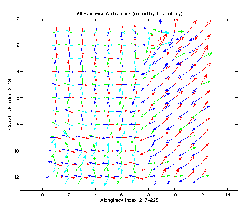
This figure shows a typical region with each of the wind ambiguities displayed at each cell. Blue is the first (most likely) ambiguity, red is the second, green the third and aqua the fourth. In order to determine an estimate of the wind across the entire swath, an ambiguity selection algorithm is needed. The Point-wise Median FilterIn order to select the proper ambiguity, we assume that the estimates are correlated from one cell to the next. In other words, we assume that the wind is unlikely to shift radically from one cell to the next. Using this assumption, we may use a variety of techniques to select a single ambiguity at each wvc. A common technique used to correlate the estimates is based on the point-wise median filter. This method does not alter any of the wind estimates generated; rather is selects between the ambiguities at each cell. Like median filters used in image processing, the point-wise median filter attempts to preserve edges and avoid blurring. The entire swath is initialized to the first ambiguity. For each cell in the swath, a 7-cell window is generated around the cell in question, and an average of all of the wind vectors is taken. The ambiguity closest to this windowed average is selected. This process is repeated until there are no more changes (or until a maximum number of iterations is achieved). |