2D Reconstruction from Irregular Samples with Variable Apertures: Software
Prof. David G. Long
Brigham Young University Center for Remote Sensing
Microwave Earth Remote Sensing (MERS) Laboratory
459 Clyde Building, Provo, Utah USA
long@ee.byu.edu
|
 |
 |
Software to accompany the paper:
D.G. Long and R.O.W. Franz, Band-Limited Signal Reconstruction from Irregular Samples with Variable Apertures, IEEE Transactions on Geoscience and Remote Sensing, to appear, doi:10.1109/TGARS.215.2501366, 2016.
Two-dimensional reconstruction:
Implements two-dimensional irregularly-spaced samples with (possible) variable apertures using the approach and notation described in Long and Franz (2016). No-aperture (equivalent to an ideal δ aperture) reconstruction as implemented in irregrecon2d.m is demonstrated in demo_irregrecon2d.m. An example of the two figures produced by this routine are shown below. Variable-aperture reconstruction is implemented in irregrecon2dAp.m and is demonstrated in demo_irregreconAp.m. Three figures are produced by this routine are shown below.
Note: unlike the one-dimensional case where the (minimum number of) samples can be anywhere in the signal period, there are constraints for full two-dimensional reconstruction: the sampling must result in a full-rank D2 matrix. A routine to test the sampling rank is provided. Note that collecting additional (disjoint) samples can often result in a full-rank matrix. Extra samples are included using least-squares psuedo-inverse techniques. Also, the implementation include an option for specifying a regularization parameter to produce more numerically stable results.
Software copyright 2015 by D.G. Long at BYU. All rights retained. Users may use and modify this software so long as the source paper above is cited. No warrantee of any kind is provided. Note: this code is designed to illustrate the method. No claims are made for its efficiency.
File listing/
 README.txt
includes notes on matlab implementation
README.txt
includes notes on matlab implementation
demo_irregrecon2d.m
demonstrates 2d sampling and reconstruction w/o aperture
demo_irregrecon2dAp.m
demonstrates 2d sampling and reconstruction w/aperture
irregrecon2d.m
2d reconstruction w/o aperature
irregrecon2dAp.m
2d reconstruction w/variable aperatures
checkrankD.m
checks the rank of a particular 2d sampling w/o aperature
checkrankD_Ap.m
checks the rank of a particular 2d sampling when variable aperatures are included
Dm.m
compute 1d M-order Dirichlet function (same as in 1d directory)
Dm2d.m
compute 2d M1,M2-order Dirichlet function
ApDm.m
compute 2d aperture-filtered M1,M2-order Dirichlet function
randsample1d.m
1d sampling routine used by demo_*.m when generating uniform and cubic lattice sampling. Can do regular or uniformly-distributed irregular sampling. (same as in 1d directory)
randsample2d.m
2d sampling routine used by demo_*.m Can do regular or uniformly-distributed irregular sampling.
test_sampling2d.m
illustrates how to generate a 2d random sampling and its sampling rank.
alternates.m
illustrates and compares alternate ways of computing reconstruction matrix.
plotlocs.m
plot 2d sampling locations. Used by test_sampling2d.m
shift2d.m
circulantly shift a matrix.
shift.m
circulantly shift a vector.
myfigure.m
Matlab utility to replace standard figure call to simplify handing of figures (calls to myfigure in demo*.m can be replaced with calls to matlab's standard "figure" command if the user does not wish to use myfigure.m) (same as in 1d directory)
demo_irregrecon2d.m and irregrecon2d.m
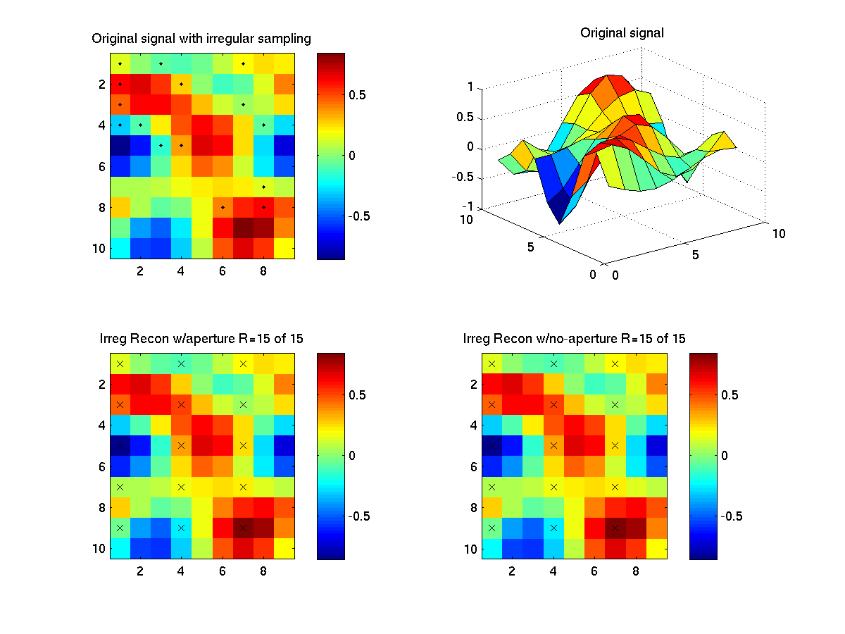
Example figures produced by demo_irregrecon2d.m: (because random number generators vary between machines, a different result will be produced for each run). This example uses no aperture function.
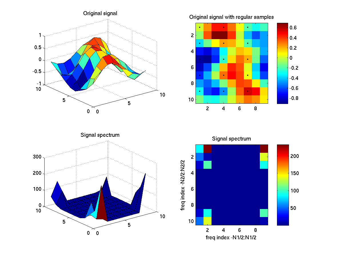
Matlab Figure 1: (upper-left panel) A bandlimited random signal is first generated. (upper-right) Same true signal as in the upper-left panel. Black dots show the locations of the regularly spaced equivalent samples. (lower-left) Power spectrum of true spectrum computed using a 2-d FFT. (lower-right) Power spectrum of the true signal computed using a 2-d FFT. This example uses M1=1, M2=2, d1=3, d2=2, resulting in a period N1=9, N2=10. Minimum number of samples is R=2(M1+1)(2M2+1)=15.
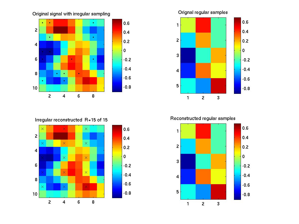
Matlab Figure 2: (upper-left panel) True signal with locations of R=15 uniformly-distributed irregular sampling locations. The irregular sampling is full-rank. (upper right panel) Values of the equivalent regular samples. (lower-right panel) Values of the irregular samples. (lower-left panel) Reconstructed signal from the irregular samples. (identical to the true signal) X's indicate the ideal regular sampling.
demo_irregrecon2dAp.m and irregrecon2dAp.m
Example figures produced by demo_irregrecon2dAp.m are: (because random number generators vary between machines, a different result will be produced for each run).
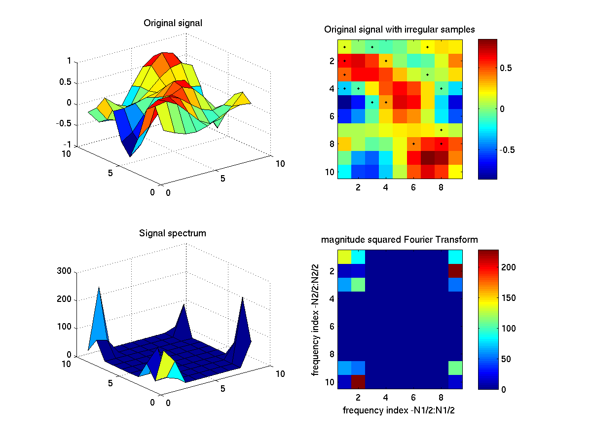
Matlab Figure 1: (upper-left panel) A bandlimited random signal is first generated. (upper-right) Same true signal as in the upper-left panel. Black dots show the locations of the regularly spaced equivalent samples. (lower-left) Power spectrum of true spectrum computed using a 2-d FFT. (lower-right) Power spectrum of the true signal computed using a 2-d FFT. This example uses M1=1, M2=2, d1=3, d2=2, resulting in a period N1=9, N2=10. Minimum number of samples is R=2(M1+1)(2M2+1)=15.
Matlab Figure 2: (upper-left panel) True signal with locations of R=15 uniformly-distributed irregular sampling locations. The irregular sampling is full-rank. (upper right panel) True signal. (lower-right panel) Reconstructed signal from the irregular samples. (identical to the true signal) X's indicate the ideal regular sampling. (lower-left panel) Same as lower-right panel.
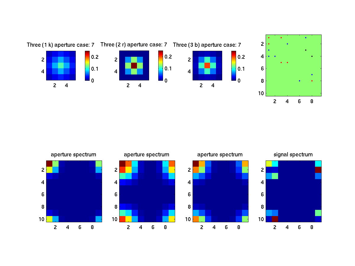
Matlab Figure 7: (left top panels) Each of the three apertures used. (right top panel) Locations of each of the irregular samples with dots color-coded to indicate which aperture is used at each sample. (lower pannels) Power spectrum of each aperture and the true signal.
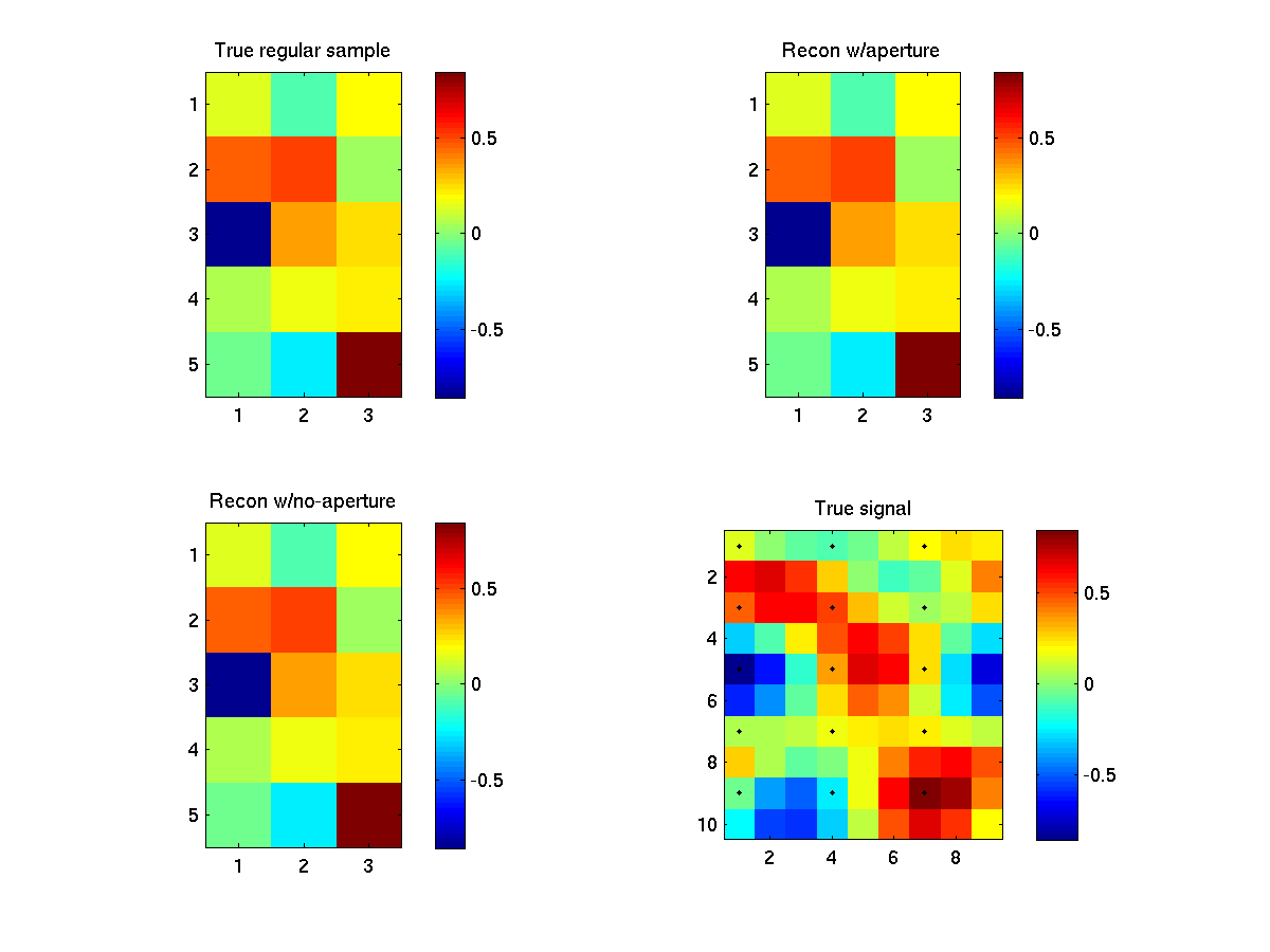
Matlab Figure 8: (upper-left panel) Sample values of the true signal at the equivalent regular sample locations. (upper-right panel) Equivalent regular sample values of the signal reconstructed from the aperture-filtered samples. Identical to upper-left. (lower-left panel) Equivalent regular sample values of the signal reconstructed from ideal apertures. Identical to upper-left. (lower-right panel) True signal with locations of equivalent regular sampling.
Maintained by David Long
long@ee.byu.edu
Last modified: 20 Nov 2015