1D Reconstruction from Irregular Samples with Variable Apertures: Software
Prof. David G. Long
Brigham Young University Center for Remote Sensing
Microwave Earth Remote Sensing (MERS) Laboratory
459 Clyde Building, Provo, Utah USA
long@ee.byu.edu
|
 |
 |
Software to accompany the paper:
D.G. Long and R.O.W. Franz, Band-Limited Signal Reconstruction from Irregular Samples with Variable Apertures, IEEE Transactions on Geoscience and Remote Sensing, to appear, doi:10.1109/TGARS.215.2501366, 2016.
One-dimensional reconstruction:
General implementation of one-dimensional reconstruction
Direct implemenation of Long and Franz (2016)
Implements one-dimensional irregularly-spaced samples with (possible) variable apertures using the approach and notation described in Long and Franz (2016). No-aperture (equivalent to an ideal δ aperture) reconstruction as implemented in irregrecon.m is demonstrated in demo_irregrecon.m. An example of the two figures produced by this routine are shown below. Variable-aperture reconstruction is implemented in irregreconAp.m and is demonstrated in demo_irregreconAp.m. Three figures are produced by this routine are shown below.
Software copyright 2015 by D.G. Long at BYU. All rights retained. Users may use and modify this software so long as the source paper above is cited. No warrantee of any kind is provided. Note: this code is designed to illustrate the method. No claims are made for its efficiency.
File listing/
 README.txt
demo_irregrecon.m
demonstrates 1d sampling and reconstruction w/o aperture
demo_irregreconAp.m
demonstrates 1d sampling and reconstruction w/variable apertures
irregrecon.m
1d reconstruction w/o aperature
irregreconAp.m
1d reconstruction w/variable aperatures
Dm.m
compute 1d M-order Dirichlet function
ApDm.m
compute 1d aperture-filtered M-order Dirichlet function
randsample1d.m
1d sampling routine used by demo_*.m Can do regular or uniformly-distributed irregular sampling.
myfigure.m
Matlab utility to replace standard figure call to simplify handing of figures (calls to myfigure in demo*.m can be replaced with calls to matlab's standard "figure" command if the user does not wish to use myfigure.m)
demo_irregrecon.m and irregrecon.m
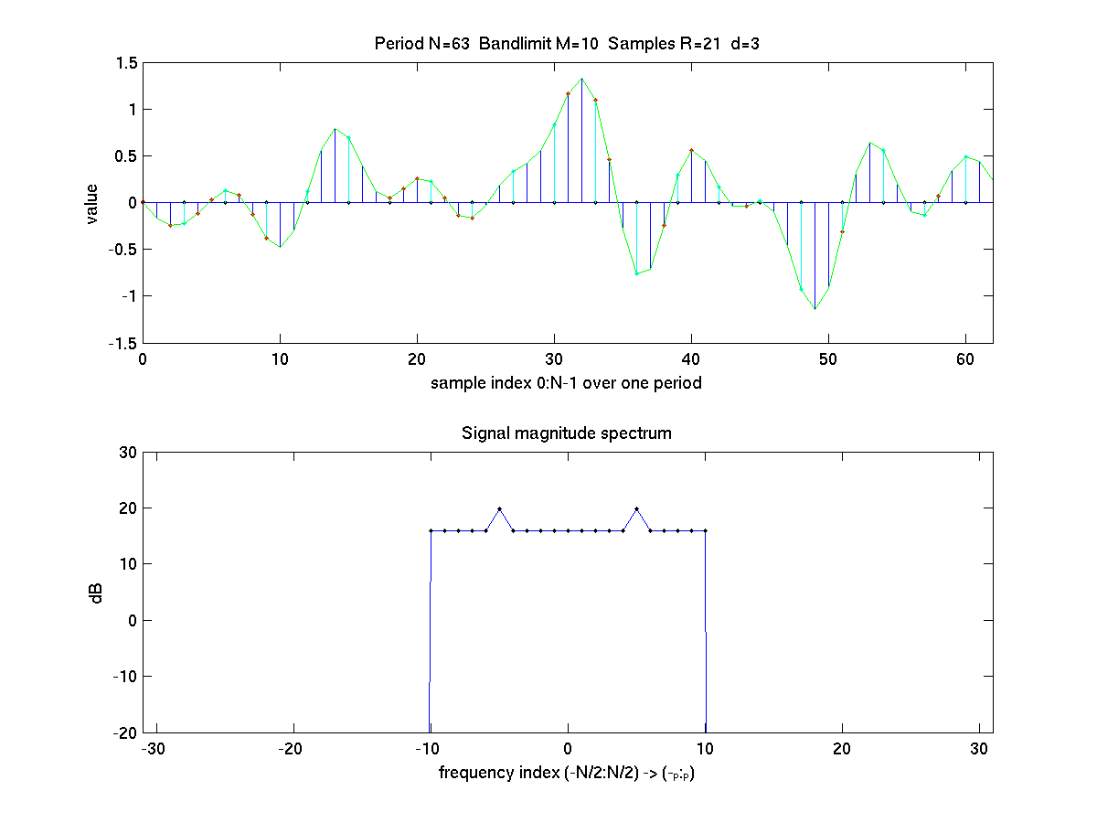
Example figures produced by demo_irregrecon.m: (because random number generators vary between machines, a different result will be produced for each run). This example uses no aperture function.
Matlab Figure 1: (top panel) A bandlimited random signal with a constant power spectrum plus an added sine wave is first generated. It is shown as the continuous green line. The (ideal) high rate sampling is the blue stem lines. Ideal regular samples (d=3) are
shown as green step lines. (Some green stem lines lie on top of blue stem lines)
The irregular random samplings is shown as red points, which in this case lie on the original signal line. The reconstructed signal computed from the irregular samples precisely overlays the original. (bottom planel) power spectrum of the original (and reconstructed) signals
This example uses M=10 and d=3 with R=2M+1=21 samples and period N=63.
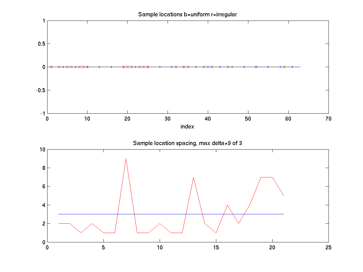
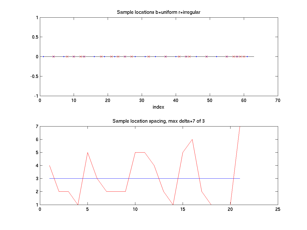
Matlab Figure 6: (top panel) Regular sample sample locations shown as blue dots on sample axes with irregular sample location shown as read x's. (bottom panel) Spacing between irregular samples (red line) and spacing between regular samples (d=3).
demo_irregreconAp.m and irregreconAp.m
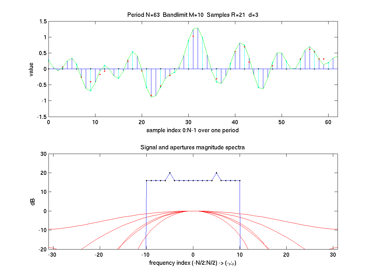
Example figures produced by demo_irregreconAp.m are: (because random number generators vary between machines, a different result will be produced for each run).
Matlab Figure 1: (top panel) A bandlimited random signal with a constant power spectrum plus an added sine wave is first generated. It is shown as the continuous green line. The (ideal) high rate sampling is the blue stem lines. Ideal regular samples (d=3) are shown as green step lines. (Some green stem lines lie on top of blue stem lines)
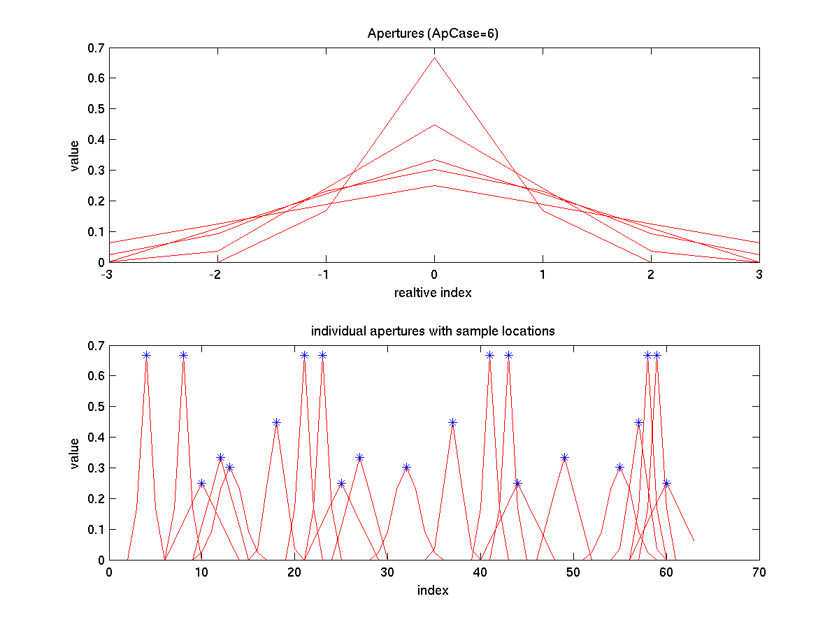
Each sample is assigned one of five different aperture functions. The irregular aperture-filtered random samples ire shown as red asterisks. Due to the aperturefunction these do not generally lie on the the original function. The reconstructed signal computed from the irregular samples precisely overlays the original. (bottom planel) power spectrum of the original (and reconstructed) signals
This example uses M=10 and d=3 with R=2M+1=21 samples and period N=63.
Matlab Figure 2: (top panel) Individual aperture functions for each sample centered at zero. These are sampled Hamming windows. The plot is clipped to +/-3 high rate samples from the aperture center. (bottom panel) Individual aperture functions for each sample centered at the sample location shown as a blue asterisk. Each aperture-filtered sample is computed by summing the values of the aperture function times time the high rate signal.
clipped.
Matlab Figure 6: (top panel) Regular sample sample locations shown as blue dots on sample axes with irregular sample location shown as read x's. (bottom panel) Spacing between irregular samples (red line) and spacing between regular samples (d=3).
Maintained by David Long
long@ee.byu.edu
Last modified: 20 Nov 2015